The problem
Utah arrays implanted in the primary visual cortex are facing the double challenge of recording a dense cortical structure, with an impedance more suited to multi-units recording. This makes it hard to obtain single unit activity (SUA), especially when the array has been implanted for quite some time. Even with the advent of high throughput template matching spike sorter (i.e. Kilosort), getting some SUA from large arrays is not trivially simple. I’ve been playing around with Kilosort 3 to get some nice SUA, and while there is no such thing as a magic combination of parameters, here are a few useful tips.
Solution part one
First things first, install Kilosort 3 following the instructions.
- Generate a channel map that linearizes the Utah array, as we don’t really care about geometry here and Utah contact sites a very distant from one another :
Nchannels = 128;
connected = true(Nchannels, 1);
chanMap   = 1:Nchannels;
chanMap0ind = chanMap - 1;
xcoords   = ones(Nchannels,1)*1000;
ycoords   = [1:Nchannels]'*1000;
kcoords   = [1:Nchannels]'; % grouping of channels (i.e. tetrode groups)

fs = 30000; % sampling frequency
save('./linear_utah_array.mat', ...
    'chanMap','connected', 'xcoords', 'ycoords', 'kcoords', 'chanMap0ind', 'fs')
- Turn off drift correction in “main_kilosort3.m”, which is useless in the given geometry :
ops.nblocks = 0; % blocks for registration. 0 turns it off, 1 does rigid registration. Replaces "datashift" optio
These two simple steps should already vastly improve Kilosort 3’s compatibility with Utah array recordings.
Soltuion part two
It’s also a decent idea to have a look at the role of the parameters when looking for SUAs. Kilosort’s code is easy to integrate into a parameter scan. Rewrite main_kilosort3.m into :
function main_ks3_scan(ops)
    % Add paths
    addpath(genpath('your_path_to_ks_folder')) % path to kilosort folder
    addpath('your_path_to_npy_matlab') % for converting to Phy

    % Set paths
    rootZ = '.\'; % the raw data binary file is in this folder
    rootH = '.\'; % path to temporary binary file (same size as data, should be on fast SSD)
    pathToYourConfigFile = '.\'; % take from Github folder and put it somewhere else (together with the master_file)
    chanMapFile = 'linear_utah_array.mat';

    ops.trange    = [0 Inf]; % time range to sort
    ops.NchanTOT  = 128; % total number of channels in your recording

    ops.fproc   = fullfile(rootH, 'temp_wh.dat'); % proc file on a fast SSD
    ops.chanMap = fullfile(pathToYourConfigFile, chanMapFile);

    % main parameter changes from Kilosort2 to v2.5
    ops.sig        = 20;  % spatial smoothness constant for registration
    ops.fshigh     = 300; % high-pass more aggresively
    ops.nblocks    = 0; % blocks for registration. 0 turns it off, 1 does rigid registration. Replaces "datashift" option.

    % Print data location
    fprintf('Looking for data inside %s \n', rootZ)

    % Check for channel map file
    fs = dir(fullfile(rootZ, 'chan*.mat'));
    if ~isempty(fs)
        ops.chanMap = fullfile(rootZ, fs(1).name);
    end

    % Find the binary file
    fs          = [dir(fullfile(rootZ, '*.bin')) dir(fullfile(rootZ, '*.dat'))];
    ops.fbinary = fullfile(rootZ, fs(1).name);

    % Run the algorithm steps
    rez                = preprocessDataSub(ops);
    rez                = datashift2(rez, 1);
    [rez, st3, tF]     = extract_spikes(rez);
    rez                = template_learning(rez, tF, st3);
    [rez, st3, tF]     = trackAndSort(rez);
    rez                = final_clustering(rez, tF, st3);
    rez                = find_merges(rez, 1);

    % Save results to Phy
    rootZ = fullfile(rootZ, 'kilosort3');
    mkdir(rootZ)
    rezToPhy2(rez, rootZ);
end
Similarly, rewrite the StandardConfig_MOVEME file into a function, then write a new matlab script :
% Load the default parameters from StandardConfig_MOVEME.m
ops = StandardConfig_MOVEME();

% Define the range of values for the lam, ThPre, and Th parameters
lam_vals = [5, 10, 20, 50];
ThPre_vals = [6, 8, 10, 12];
Th_vals = [8 4; 10 4; 12 4; 14 4];

% Initialize a structure to store the results

% Initialize the result index
result_idx = 1;

% Perform the parameter sweep
for lam_idx = 1:length(lam_vals)
    for ThPre_idx = 1:length(ThPre_vals)
        for Th_idx = 1:size(Th_vals, 1)
            % Update the lam, ThPre, and Th parameter values
            ops.lam = lam_vals(lam_idx);
            ops.ThPre = ThPre_vals(ThPre_idx);
            ops.Th = Th_vals(Th_idx, :);

            % Run the mainFunction with the updated ops and store the results
            main_ks3_scan(ops);
            fprintf('lam: %d, ThPre: %d, Th: [%d, %d]\n', ops.lam, ops.ThPre, ops.Th(1), ops.Th(2));
            fprintf('--------------');

        end
    end
end
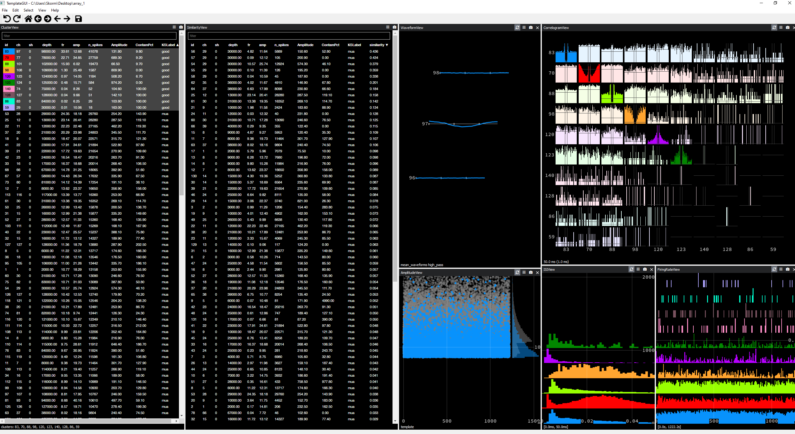
This yields a number of good clusters w.r.t. spike-sorting parameters. However, more is not always better, as instances where the number of clusters is maximum are often obtained through low stringency on the thresholds, and end up giving poorly clustered units with few spikes. Similarly, with a low lam parameter, low amplitude (artifactual ?) clusters tend to show up a lot.
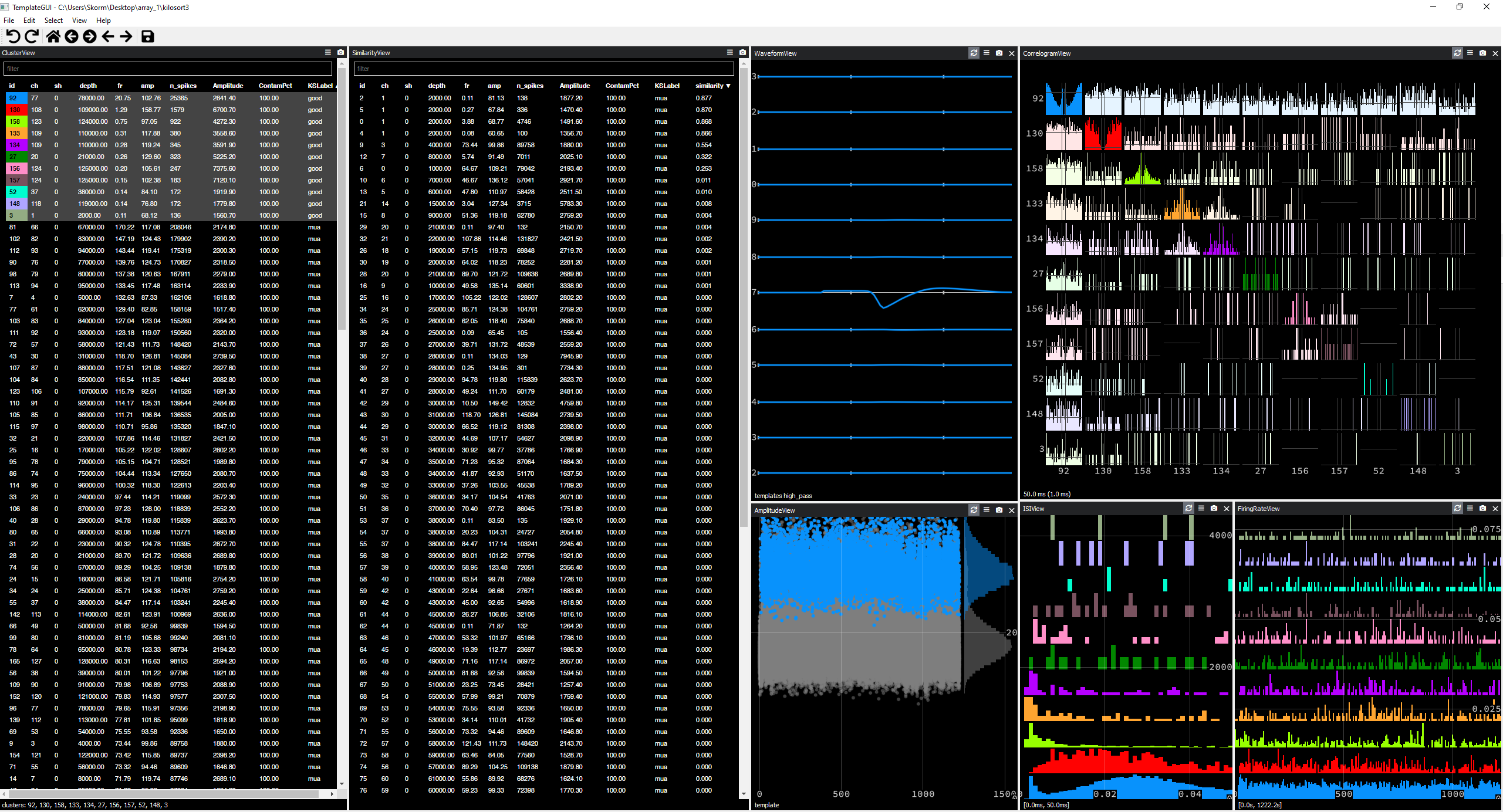
By manually visualizing the clusters with Phy, I ended up settling with parameters lam = 10 ; ThPre = 10 ; Th = [12 6], which yields nicer single units :
This is not a miracle solution, but it ends up offering similar performance to what Kilosort 2 used to output, whilst doing a better job at tracking the MUAs than KS2. If a miracle solution does show up, I’ll make another post !
